Spectral PSF Model Product

Metadata

Data product name	DpdSirSpectralPsfModel
Data product custodian	SIR
Name of the Schema file	euc-sir-SpectralPsfModel.xsd
Processing function using the data product	SIR

Proposed for inclusion in EAS/SAS

This product is proposed for inclusion in the SAS: no

This is an internal Data Product.

Data product elements

Header	object of type sys:genericHeader
Data	object of type sir:sirSpectralPsfModel
QualityFlags	object of type dqc:sqfPlaceHolder
Parameters	object of type ppr:genericKeyValueParameters

Detailed description of the data product

The sirSpectralPsfModel describes the 2D spectrogram width across the ideal dispersion direction, which (in case GWA_TILT=0) is perfectly aligned along the pixels grid. The model operates within the SIR rotated layout where the dispersion direction is nearly horizontal, and this direction remains consistent across all detectors (see Optical Model Product description for further details).

The Curvature Model Product describes the geometric curvature of spectrograms and its variation within the Field of View (FoV); similarly, the sirSpectralPsfModel describes the chromatic evolution of the cross-dispersion width (in pixels), as well as its variations within the FoV.

Each grism/tilt configuration is independently calibrated and the coefficients of each configuration are stored in the sirPsfModelOrders structure. The sirPsfModel collects all the sirPsfModelOrders available.

Relevant items of sirPsfModelOrder, are (see Fig. 36, and Fig. 34 for additional details):

• GWATilt: the grism nominal tilt value (0, +4, -4);

• ExtraTilt: the extra tilt computed during calibration (not implemented yet);

• SpectraOrder: the list of sirPsfModelContent, each item contains the geometrical description of a given spectrum order for the current grism (see description below).

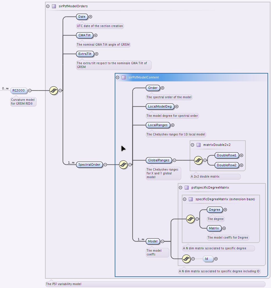
Fig. 36 The DpdSirSpectralPsfModel description.

Cross-dispersion width measurement

The cross-dispersion width is estimated from (unsaturated) spectrograms of bright stars within the FoV, using a Gaussian-fit of the cross-dispersion profile (actually an erf-fit to account for integration over pixels and minimize sub-sampling issue if any).

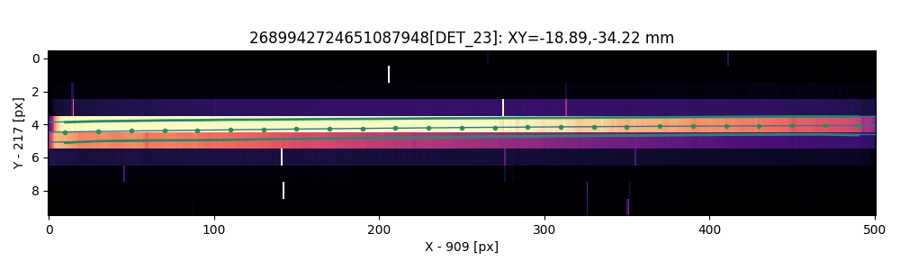
Fig. 37 An RGS000+0 spectrogram, shown in SIR coordinates (pixels). Obviously, along-dispersion axis is horizontal, while cross-dispersion axis is vertical.

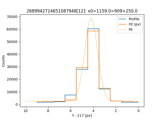
Fig. 38 A cross-dispersion profile, and the Gaussian fit used to estimate the cross-dispersion position and width of the spectrogram at given along-dispersion position.

SpectraOrder description

For each spectrogram and dispersion order, a 1D-Chebychev polynomial expansion (of order \(N\)) is used to model the cross-dispersion width \(\sigma\) (in pixel), as a function of the distance \(\Delta d\) (in mm) from the reference position set by the sirOptModel (see Fig. 39):

(6)\[\sigma \text{[pix]} \approx \sum_{k=0}^N \alpha_{x,y,k} T_k\left(\Delta d \text{[mm]}\right)\]

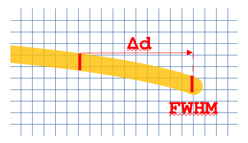
Fig. 39 The spectrogram width and its description according with the PsfModel.

This is the so-called local model. Each spectrogram, probing different positions \((x, y)\) in the FoV, has its own set of coefficients \(\alpha_{x,y,k=0\ldots N}\).

The SIR Pipeline then uses a global model to describe the spatial variations of the local coefficients \(\alpha\) across the FoV, namely a 2D Chebychev polynomial expansion:

\[\alpha_{x,y,k} \approx \sum_{i,j} a^{(k)}_{i,j} T_i(x)T_j(y)\]

These \(\textbf{A}^{(k)} := \{ a^{(k)}_{i,j} \}\) matrices are stored in the sirPsfModelContent structure, which contains (see Fig. 36 and Fig. 34 for additional details):

• Order: the order of the spectrum (1st, 0th, 2nd, …) to be described;

• LocalModelDeg: the degree of the Local crv model (\(N\) in the equation (6));

• LocalRanges: the validity domain of the local Chebychev polynomial; this range plays the same rule of the domain variable in numpy.polynomial.chebyshev.Chebyshev definition. (Range extremes are in mm)

• GlobalRanges: the validity domain (along the 2 directions of the FoV) of the local 2D Chebychev polynomial. Even in the case the range extremes are in mm

• Model: a list of specificDegreeMatrix, each item of this list contains one \(\textbf{A}^{(k)}\) matrix. If the local polynomial is of degree \(N\), the model will contain \(N+1\) matrices. Each matrix is used to obtain one local coefficient \(\alpha_{x,y,k}\) in a given position \((x,y)\) of the FoV.